Visibility Settings
|
1238888 |
The views can also show objects other than the scan points, such as:
- The positions of the other scans in the project.
- The simple objects assigned to a scan that were created by a fit, for example spheres, and 3D points.
- CAD models.
Not all views can display all these objects. For further information, see the more detailed description of views.
You can decide whether to display the objects using the visibility settings, which are arranged in three levels:
- The visibility of the layer to which the object is assigned.
- The visibility according to the prominence of the object.
- The distance of the object from the observer.
An object is only visible if the visibility on the first two levels is set accordingly and it is located in the set range.
The visibility settings are maintained separately for each view. It is therefore possible that an object is visible in one view and not in another. When you open a new view, this view initially takes over the default values of the visibility settings. You can also change these default values.
Right-click in a view in the work area, then select Visibility Settings. The Visibility Settings dialog is displayed.
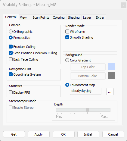
Figure 10-65 Visibility settings in 3D view
General
Camera
Only available in the 3D view. You can select Orthographic or Perspective.
-
Orthograpic: 3D elements are presented in a 2D perspective.
-
Perspective: The site is displayed in complete 3D as if you were on site.
Culling Options
There are several options to hide objects and scan points to reduce the rendering load and make navigation smoother.
-
Frustrum Culling: Hides objects outside the camera's field of vision.
-
Scan Position Occlusion Culling: Hides scan positions that are not visible from the your current angle.
-
Backface Culling: Hides the backface of points, see Backface Culling.
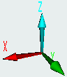
Navigation Hint
Displays or hides the coordinate system.
Render Mode
Select whether you want to display 3D elements with wireframe, smooth shading or both.
Background
Select the 3D view background. This can be either a color gradient or an environment map. For further information, see Environment Map as Background Image for a 3D View.
Statistics
Displays the frames per second.
Stereoscopic Mode
If enabled, 3D scan data is displayed from two slightly offset viewpoints to create a depth‑enhanced, three‑dimensional visualization on supported 3D‑enabled displays and in VR. By means of the Depth slider you can modify the depth enhancement.
View (3D View only)
If Auto apply changes is selected, new settings are visible immediately; you do not need to click the Apply button.
Quality Settings
Determines the image quality while moving.
If the handle of the slider is moved to the left, the quality of the rendering is reduced during movement in favor of performance.
If the handle of the slider is moved to the right, the quality increases and the performance decreases. If the handle of the slider is moved completely to the right, there will be no quality penalty during movement.
Clear View Settings
In the clear view mode, points in areas with low point density will be displayed more transparently and points in areas with a high point density will be displayed more brightly.
Enable Clear View: Check if you want to use Clear View. By changing the settings with the Transparency slider you can intensify or weaken this effect.
Gap Filling
Fills gaps between scan points that are physically close to each other.
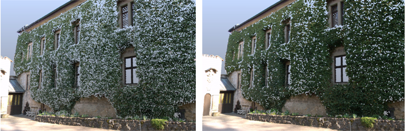
Figure 10-66 Gap filling turned off (left) and turned on (right)
If clear view and gap filling are grayed out, Offscreen Rendering under Tools > Options > View might be disabled. Offscreen Rendering must be enabled for Gap Filling and Clear View.
Supersampling
Renders the point cloud with a resolution higher than the resolution of your screen and then shrinks the point cloud to fit the screen resolution. This reduces anti-aliasing effects and gives the point cloud a smoother visual appearance. Fine and filigree structures look sharper and stray points will appear less annoying. Set the resolution of the initially rendered point cloud compared to the screen resolution by selecting one of the options 2x2, 3x3, or 4x4. For example, choosing 2x2 means that the point cloud will be rendered with a resolution that is 4 times the resolution of your screen.
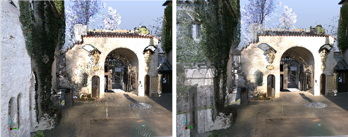
Figure 10-67 Supersampling turned off (left) and turned on (right)
Objects like walls might appear transparent when using small point sizes in combination with supersampling. High supersampling resolutions like 4x4 require large amounts of graphics card memory.
Scan Points (3D View only)
If Auto apply changes is selected, new settings are visible immediately; you do not need to click the Apply button.
Point Size
-
Fixed: Keeps all points at the same pixel size regardless of their distance from the viewpoint.
-
Adaptative: Automatically adjusts the visual size of points depending on their distance from the viewpoint.
Color Settings
You can determine how scan points will be colored. Note that these settings do not work in Orbis and Blink projects.
-
Measured Value: Scan points will be displayed in the original colors.
-
White: Scan points will be displayed white.
-
Black: Scan points will be displayed black.
-
Unique for Scans: Colors each scan in a unique color.
-
Unique for Clusters: Colors each cluster in a unique color.
Coloring (3D View only)
The coloring tab lets you set values that are used in coordinate coloring. For more information, see Coloring.
Reference Object
Reference is the object used as a reference for coloring x, y, z, xyz, and distance. The reference object can be scan origin, clipping box, or marked point. If you choose custom, you can define the reference origin to be anywhere, even where no point exists.
Reference Origin
Only active if you selected custom as your reference origin.
Use local coordinates
Only available in the 3D view. If activated, the local coordinates are used.
Coloring Ranges
Minimum and maximum values are required in order map the data to colors. A larger gap between the minimum and maximum value makes the bands of color larger. Points outside the minimum and maximum are colored the same as minimum and maximum.
Use active clipping boxes: Creates a temporary clipping box that is large enough to contain all the clipping boxes that are active in the project, then sets the origin and ranges to apply coloring within the confines of the new clipping box.
Blend point color with coloring
The original colors of the scan points can be blended with the colors produced by coordinate coloring to give a shading. This helps to retain the original features of the scan, while still getting the additional information provided by coordinate coloring.
Colormap
Choose the color map for coloring. Choices are:
-
Rainbow
-
Cold-Hot, which is blue, white and red values
-
Linear, which is black increasing to red (x), green (y), blue (z) and white (distance)
Select Discrete if you want to have solid colors instead of continuous colors. Use Increments to set the number of discrete colors.
Shading (3D View only)
For more information, see Coloring.
-
Shading Strength: Increases or decreases the strength of shading.
-
Apply to: You can apply shading to Points, Meshes or Both.
Layer
Toggle the visibility of the available layers and their related objects and the object names in the view.
Extra
Objects
Display or hide certain types of objects:
-
Models Folder : Display CAD models.
-
References Folder: Display reference objects.
-
Scan positions: Display the scanner positions in the view. For more information on the icons representing different scan types, see Scanner Icons in the 3D View.
-
Cameras: Only available in the 3D view. Display the camera positions of other views.
Scan objects
Display or hide the objects that are assigned to the scans in the view. You may display these objects only if the scan is loaded. The When loaded only checkbox is only available in the 3D view.
Visibility
Set the minimum and maximum distance at which objects are shown.
Labels
Set the maximum distance at which the labels of annotations are shown.